Solvation energies
Solvation energies are usually decomposed into a free energy cycle as shown in the free energy cycle below. Note that such solvation energies often performed on fixed conformations; as such, they are more correctly called “potentials of mean force”. More details on using APBS for the polar and nonpolar portions of such a cycle are given in the following sections.
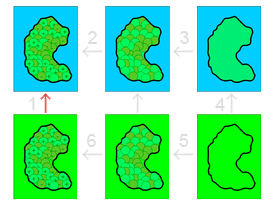
Our model solvation free energy cycle illustrating several steps:
- The solvation energy to be calculated.
- Charging of the solute in solution (e.g., inhomogeneous dielectric, ions present).
- Introduction of attractive solute-solvent dispersive interaction interactions (e.g., an integral of Weeks-Chandler-Andersen interactions over the solvent-accessible volume).
- Introduction of repulsive solute-solvent interaction (e.g., cavity formation).
- Basically a null step although it could be used to offset unwanted energies added in Steps 3 and 4 above.
- Charging of the solute in a vacuum or homogeneous dielectric environment in the absence of mobile ions.
Polar solvation
The full free energy cycle is usually decomposed into polar and nonpolar parts. The polar portion is usually represented by the charging energies in Steps 2 and 6:
Energies returned from APBS electrostatics calculations are charging free energies. Therefore, to calculate the polar contribution to the solvation free energy, we simply need to setup two calculations corresponding to Steps 2 and 6 in the free energy cycle. Note that the electrostatic charging free energies returned by APBS include self-interaction terms. These are the energies of a charge distribution interacting with itself. Such self-interaction energies are typically very large and extremely sensitive to the problem discretization (grid spacing, location, etc.). Therefore, it is very important that the two calculations in Steps 2 and 6 are performed with identical grid spacings, lengths, and centers, in order to ensure appropriate matching (or “cancellation”) of self-energy terms.
Born ion
One of the canonical examples for polar solvation is the Born ion: a nonpolarizable sphere with a single charge at its center surrounded by an aqueous medium. Consider the transfer of a non-polarizable ion between two dielectrics. In the initial state, the dielectric coefficient inside and outside the ion is \(\epsilon\_{\mathrm {in}}\), and in the final state, the dielectric coefficient inside the ion is \(\epsilon\_{\mathrm {in}}\) and the dielectric coefficient outside the ion is \(\epsilon\_{\mathrm {in}}\). In the absence of external ions, the polar solvation energy of this transfer for this system is given by:
where q is the ion charge, a is the ion radius, and the two ε variables denote the two dielectric coefficients. This model assumes zero ionic strength.
Note that, in the case of transferring an ion from vacuum, where \(\epsilon\_{\mathrm {in}} = 1\), the expression becomes
We can setup a PQR file for the Born ion for use with APBS with the contents:
REMARK  This is an ion with a 3 A radius and a +1 e charge
ATOM      1   I  ION     1 0.000   0.000   0.000  1.00 3.00
We’re interested in performing two APBS calculations for the charging free energies in homogeneous and heterogeneous dielectric coefficients. We’ll assume the internal dielectric coefficient is 1 (e.g., a vacuum) and the external dielectric coefficient is 78.54 (e.g., water). For these settings, the polar Born ion solvation energy expression has the form
where z is the ion charge in electrons and R is the ion size in Å.
This solvation energy calculation can be setup in APBS with the following input file:
# READ IN MOLECULES
read
  mol pqr born.pqr
end
elec name solv # Electrostatics calculation on the solvated state
  mg-manual # Specify the mode for APBS to run
  dime 97 97 97 # The grid dimensions
  nlev 4 # Multigrid level parameter
  grid 0.33 0.33 0.33 # Grid spacing
  gcent mol 1 # Center the grid on molecule 1
  mol 1 # Perform the calculation on molecule 1
  lpbe # Solve the linearized Poisson-Boltzmann equation
  bcfl mdh # Use all multipole moments when calculating the potential
  pdie 1.0 # Solute dielectric
  sdie 78.54 # Solvent dielectric
  chgm spl2 # Spline-based discretization of the delta functions
  srfm mol # Molecular surface definition
  srad 1.4 # Solvent probe radius (for molecular surface)
  swin 0.3 # Solvent surface spline window (not used here)
  sdens 10.0 # Sphere density for accessibility object
  temp 298.15 # Temperature
  calcenergy total # Calculate energies
  calcforce no # Do not calculate forces
end
elec name ref # Calculate potential for reference (vacuum) state
  mg-manual
  dime 97 97 97
  nlev 4
  grid 0.33 0.33 0.33
  gcent mol 1
  mol 1
  lpbe
  bcfl mdh
  pdie 1.0
  sdie 1.0
  chgm spl2
  srfm mol
  srad 1.4
  swin 0.3
  sdens 10.0
  temp 298.15
  calcenergy total
  calcforce no
end
# Calculate solvation energy
print energy solv - ref end
quit
Running this example with a recent version of APBS should give an answer of -229.59 kJ/mol which is in good agreement with the -230.62 kJ/mol predicted by the analytic formula above.
Note
The Born example above can be easily generalized to other polar solvation energy calculations. For example, ions could be added to the solv ELEC, dielectric constants could be modified, surface definitions could be changed (in both ELEC sections!), or more complicated molecules could be examined. Many of the examples included with APBS also demonstrate solvation energy calculations.
Note
As molecules get larger, it is important to examine the sensitivity of the calculated polar solvation energies with respect to grid spacings and dimensions.
Apolar solvation
Referring back to the solvation free energy cycle, the nonpolar solvation free energy is usually represented by the energy changes in Steps 3 through 5:
where Step 4 represents the energy of creating a cavity in solution and Steps 3-5 is the energy associated with dispersive interactions between the solute and solvent. There are many possible choices for modeling this nonpolar solvation process. APBS implements a relatively general model described by Wagoner and Baker (2006) and references therein. The implementation and invocation of this model is described in more in the APOLAR input file section documentation. Our basic model for the cavity creation term (Step 4) is motivated by scaled particle theory and has the form
where \(p\) is the solvent pressure (press keyword), \(V\) is the solute volume, \(\gamma\) is the solvent surface tension (gamma keyword), and \(A\) is the solute surface area.
Our basic model for the dispersion terms (Steps 3 and 5) follow a Weeks-Chandler-Anderson framework as proposed by Levy et al (2002):
where \(\overline{\rho}\) is the bulk solvent density (bconc keyword), \(\Omega\) is the problem domain, \(u^{\mathrm{(att)}}(y)\) is the attractive dispersion interaction between the solute and the solvent at point y with dispersive Lennard-Jones parameters specified in APBS parameter files, and \(\theta(y)\) describes the solvent accessibility of point y.
The ability to independently adjust press, gamma, and bconc means that the general nonpolar solvation model presented above can be easily adapted to other popular nonpolar solvation models. For example, setting press and bconc to zero yields a typical solvent-accessible surface area model.